Notebooks

The notebooks component of OpenHEXA is a customized Jupyter deployment.

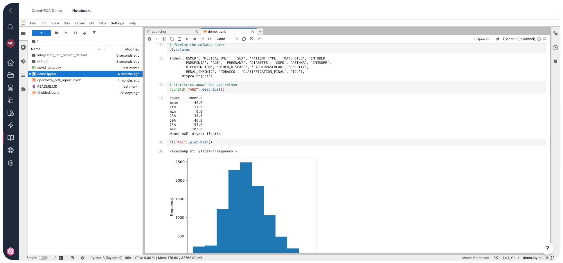
Jupyter is a flexible integrated development environment built around notebooks—documents that combine code, documentation, data, and rich visualizations. It provides a fast interactive environment for prototyping and explaining code, exploring and visualizing data, and sharing ideas with others. For more information about the Jupyter stack, see the official Jupyter documentation.

Notebook permissions by role

Viewers: Cannot access or use notebooks
Editors and Admins: Can launch and use the Jupyter notebook environment

Use cases¶

You can use notebooks in OpenHEXA for various purposes:

Explore and perform preliminary analysis of a dataset
Explain and illustrate an algorithm or a data model in a literate programming style
Prototype a visualization dashboard
Create a simple data pipeline

When to use pipelines instead¶

Consider using OpenHEXA data pipelines instead when you want to:

Let non-technical users launch data processing workflows using a web interface
Schedule a data workflow to run at specific times
Apply standard software development practices like version control or unit tests

OpenHEXA notebook features¶

The OpenHEXA notebooks component works as a standard Jupyter environment, with a few helpful additions:

Many pre-installed libraries
Access to the shared workspace filesystem in the Jupyter file browser
Workspace database credentials automatically exposed as environment variables

This guide walks you through the specifics of the OpenHEXA notebooks environment. You may also find these guides helpful:

Using the OpenHEXA SDK: The OpenHEXA SDK is a Python library that provides building blocks and helper methods for writing code on OpenHEXA
Using the OpenHEXA Toolbox: The OpenHEXA Toolbox is a collection of utilities that can help you with health data science integration and analysis workflows

Key JupyterLab features¶

JupyterLab provides a powerful interface for data science work. Here are some of the most important features you'll use:

The left sidebar has a file browser that gives you access to your workspace files. You can: - Navigate through directories by clicking folder names - Create new files and folders using the + button - Upload files by dragging and dropping them into the browser - Right-click files to access context menus for renaming, deleting, or downloading

Cell types and execution¶

Notebooks are made up of cells that can contain different types of content: - Code cells: Execute Python, R, or other programming languages - Markdown cells: Write formatted text, documentation, and explanations - Raw cells: Plain text that won't be processed

Use Shift + Enter to execute a cell and move to the next one, or Ctrl + Enter to execute without moving.

Variable inspector¶

The variable inspector (accessible from the left sidebar) shows all variables currently in memory, their types, and values. This is particularly useful for: - Debugging your code - Understanding data structures - Monitoring memory usage - Exploring datasets interactively

Command palette¶

Press Ctrl + Shift + C (or Cmd + Shift + C on Mac) to open the command palette, which provides quick access to: - All available commands and shortcuts - File operations - Cell operations - Extension features

Split view and tabs¶

JupyterLab supports multiple views of your work: - Split view: Drag tabs to create side-by-side or stacked layouts - Multiple tabs: Open several notebooks or files at the same time - Tab management: Right-click tabs for options like Close All or Close Others

Keyboard shortcuts¶

Essential shortcuts for efficient work: - A / B: Insert cell above or below - DD: Delete cell - M / Y: Change cell to Markdown or Code - Shift + M: Merge cells - Ctrl + S / Cmd + S: Save notebook - Z: Undo cell deletion

Use the workspace filesystem¶

When you launch the notebooks environment, you'll see that the Jupyter filesystem displays two directories:

The tmp directory
The workspace directory

You can only write data in these two directories. You can't create files or directories at the root of the filesystem.

For more information about the workspace and tmp directories and how to use them with Python, see the SDK documentation. For R users, see the code sample below (we don't have an SDK for R yet).

https://github.com/BLSQ/openhexa/assets/690667/8f279c1f-c371-490f-a04f-84a97b028859

Here is a basic example showing how to read / write data to the workspace filesystem in Python:

import pandas as pd
from openhexa.sdk import workspace

# Read data
df = pd.read_csv(f"{workspace.files_path}/covid_data.csv")

# Write data
df = pd.DataFrame({"foo": [1, 2, 3], "bar": [4, 5, 6]})
df.to_csv(f"{workspace.files_path}/foobar.csv")

The equivalent R example (until we have a SDK for R, you will have to hard-code the workspace directory path):

# Read data
df <- read.csv("/home/hexa/workspace/covid_data.csv")

# Write data
x          <- 1:10
y          <- letters[1:10]
some_data <- tibble::tibble(x, y)
write.csv(some_data, "foobar.csv")

https://github.com/BLSQ/openhexa/assets/690667/49e53c15-c251-4283-9450-94ae9bdff9b6

Use the workspace database¶

The workspace database is a standard PostgreSQL database. You can use any library that supports PostgreSQL to access it in a notebook.

If you use Python, the recommended way to get the database credentials is by using the OpenHEXA SDK.

Here is a minimal Python example (with SQLAlchemy) to get you started:

import pandas as pd
from sqlalchemy import create_engine, Integer
from openhexa.sdk import workspace

# Create a SQLAlchemy engine
engine = create_engine(workspace.database_url)

# Read data
pd.read_sql("SELECT * FROM covid_data", con=engine)

# Write data
df = pd.DataFrame({"foo": [1, 2, 3], "bar": [4, 5, 6]})
df.to_sql("a_new_table", con=engine, if_exists="replace", index_label="id", 
          chunksize=100, dtype={"id": Integer(), "foo": Integer(), "bar": Integer()})
pd.read_sql("SELECT * FROM a_new_table", con=engine)

Note that we use the optional chunksize and dtype arguments. Use chunksize to control the number of rows written in each batch (to optimize memory usage), and use dtype to explicitly specify PostgreSQL column types and avoid conversion issues caused by the default type guessing behavior.

Since we don't have an SDK for R yet, you'll need to use environment variables to get the database credentials when using R.

Here is how you can do it using DBI:

# Initial connection
library(DBI)
con <- dbConnect(
    RPostgres::Postgres(),
    dbname = Sys.getenv("WORKSPACE_DATABASE_DB_NAME"),
    host = Sys.getenv("WORKSPACE_DATABASE_HOST"),
    port = Sys.getenv("WORKSPACE_DATABASE_PORT"),
    user = Sys.getenv("WORKSPACE_DATABASE_USERNAME"),
    password = Sys.getenv("WORKSPACE_DATABASE_PASSWORD")
)

# Write data
x          <- 1:10
y          <- letters[1:10]
some_data <- tibble::tibble(x, y)
dbWriteTable(con, "another_table", some_data, overwrite=TRUE)
df <- dbReadTable(con, "another_table")

Use connections¶

Once you've added a new connection, you can access its parameters in your Jupyter environment through the SDK.

For more information about how to use connections in Python, see the OpenHEXA SDK documentation. For general information about connections, see the User manual.

Here's how you can access connection parameters using Python:

import os
from openhexa.sdk import workspace

print(workspace.get_connection("connection-identifier"))

Restart your Jupyter server¶

You might need to restart your Jupyter server in a few situations, such as:

Your server is completely stuck and restarting it is your last option

Unfortunately, restarting your Jupyter server isn't straightforward at the moment. We'll improve this in the future.

For now, you need to:

Open the JupyterHub control panel (File > Hub Control Panel—this opens in a new window or tab).
Find your server in the list of running servers. Each server in the list corresponds to a workspace. The server you're looking for is in the "running" state, and its name should match the URL in your browser address bar.
Click stop.
Close the Hub Control panel tab, go back to the OpenHEXA notebooks screen, and reload the page.

Tips and tricks¶

This section has a few recipes that you might find useful.

Use s3fs to interact with an S3 bucket¶

If you need to browse, download, or upload data in an Amazon S3 bucket, first add an AWS S3 connection.

Once you've added the connection, you can interact with the bucket in a Jupyter notebook.

While your OpenHEXA Jupyter environment comes with boto3 pre-installed, s3fs is easier for most operations (s3fs is also pre-installed in your environment).

Here is a basic example showing how to use s3fs in an OpenHEXA notebook:

import os
import s3fs

# The environment variable names can be copy-pasted from the connection detail page
fs = s3fs.S3FileSystem(key=os.environ["BUCKET_CONNECTION_ACCESS_KEY_ID"], secret=os.environ["BUCKET_CONNECTION_ACCESS_KEY_SECRET"])
bucket_name = os.environ["BUCKET_CONNECTION_BUCKET_NAME"]

# List the files in a directory within the bucket
fs.ls(f"{bucket_name}/data/climate")

# Download all the files from the bucket directory in the workspace filesystem
fs.get(f"{bucket_name}/data/climate", "/home/hexa/workspace/climate_data", recursive=True)

Use gcsfs to interact with a Google Cloud Storage bucket¶

If you need to browse, download, or upload data in a Google Cloud Storage bucket, first add a GCS connection.